Estimation of the frequency of neurocysticercosis among people with headache
Author
Mohammad Shah Jalal, Université de Montréal
Published
January 11, 2025
Before talking about Bayesian binomial model, let’s review some important concepts.
Binomial distribution
The binomial distribution describes the probability of observing a certain number of successes in a fixed number of independent trials, each with the same probability of success. The binomial distribution is frequently used to model the number of successes in a sample drawn with replacement (that is important) from a population.
In simpler terms, it’s used when you have an experiment that:
Is repeated a fixed number of times.
Has only two possible outcomes on each trial or test (Sick vs. Healthy).
Has the same probability of success on each trial or test.
Has independent trials (the outcome of one trial or test doesn’t affect the others)
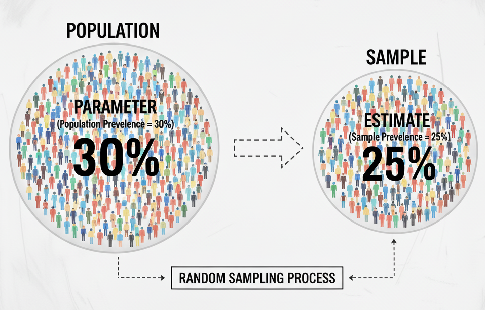
Let’s walk through a simple example. Suppose we want to estimate the prevalence of Disease X—that is, the proportion of people in Montréal, Canada, in the year 2025 who have the disease at a specific point in time. The true prevalence in the entire population (often referred to as the parameter) is unknown. Since it is not practical to test every individual living in Montréal, we instead collect data from a sample of the population and use that sample to estimate the true prevalence.
Figure: Population vs Sample
Let’s assume we randomly select 1,000 individuals from the population and test them. This situation fits perfectly within a binomial distribution framework because:
Binary outcome: Each test has only two possible results — the person is Sick (has the disease) or Healthy (does not have the disease).
Fixed number of trials: The number of tests, n, is fixed at 1,000.
Independence: One person’s disease status does not influence another’s (assuming no outbreak cluster or transmission within the sample).
Constant probability: Every individual has the same underlying probability, p, of having the disease
If 30 people test positive, then we have observed y = 30 “Sick” outcomes. The full range of possible outcomes (from 0 to 1,000 positive results), along with their corresponding probabilities, forms a binomial distribution.
So, what is the prevalence estimate for the above example?
Answer:
Code
## So, we have - y <-30# Number of people with diseasen <-1000# Number of people tested## Prevalence of X disease in MontréalPrevalence <- y/nPrevalence
[1] 0.03
Code
## If we want to express in percentage
paste0("Prevalence of X disease: ",Prevalence*100,"%")
[1] "Prevalence of X disease: 3%"
So, we can say that the prevalence of disease X in the population of Montréal is 3%.
However, this interpretation is incomplete. Because, a single proportion estimate does not account for uncertainty — such as random sampling variation, test accuracy, or selection bias. In practice, we want to quantify this uncertainty by constructing a confidence interval (CI) around our estimate. This uncertainty reflects how confident we are that the true prevalence in the population lies within a certain range.
There are several ways to calculate confidence intervals (CIs), such as the Wald approximation, Wilson method, and Clopper–Pearson method.
Let’s calculate CI for our prevalence estimate,
Code
binom.test(y, n, conf.level =0.95)
    Exact binomial test

data:  y and n
number of successes = 30, number of trials = 1000, p-value < 2.2e-16
alternative hypothesis: true probability of success is not equal to 0.5
95 percent confidence interval:
 0.02033049 0.04255140
sample estimates:
probability of success
                  0.03
Now, we can say that “The prevalence of X disease in the population of Montréal is 3% (95% CI: 2% – 4%)”.
What does this mean?
This result means the following:
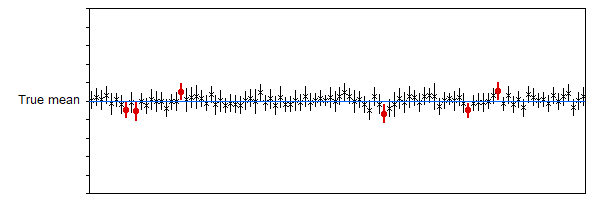
If we were to repeat this same study many times — each time randomly selecting 1000 individuals and calculating a 95% confidence interval — then approximately 95% of those intervals would contain the true population prevalence, while 5% would not.
In other words, the method we used to construct the interval has a long-run success rate of 95% in capturing the true value.
Figure: 95% confidence interval visualization
However, for our single study, we cannot say with certainty whether the true prevalence lies inside or outside this particular interval — we only know that the procedure has a 95% chance of producing a correct interval over many repetitions.
😔
That’s not quite what we usually want to know, is it?
In practice, we often wish to make a direct probability statement about the true prevalence, such as:
“We are 95% confident that the true prevalence lies between 2% and 4%.”
Unfortunately, this statement is not technically correct for our previous analysis.
Why?. Because the true prevalence is fixed — it’s not something that changes from one study to another. The uncertainty lies in our sample, NOT in the parameter itself.
Of note, the analysis we performed so far represents the frequentist approach to estimating prevalence for binomial data.
There is another powerful framework called the Bayesian approach, which allows us to directly express uncertainty about the parameter itself — for example, by saying that the probability of the prevalence being between 2% and 4% is 95%.
This interpretation aligns much better with how researchers naturally think about uncertainty.
How Bayesian statistics work?
Bayesian statistics provide a way to update our beliefs about an unknown parameter (such as disease prevalence) based on observed data.
It starts with a prior distribution, which represents what we believe about the parameter before seeing the data (for example, previous studies might suggest the prevalence is around 5%).
Where can we get prior information? - From previous studies, reasonable guesses from experts, or we can simply say that “we don’t know.”
Does the prior influence the final results? - Yes — it matters when the data are weak, and not much otherwise.
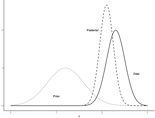
Then, we collect new data (e.g., 30 positive cases out of 1000 tests), and use Bayes’ theorem to combine this prior information with the data’s likelihood.
The result is a posterior distribution — a new, updated belief about the parameter after considering the data.
Figure: Prior, likelihood and posterior distribution.
From the posterior, we can calculate a credible interval, which gives the range of values within which the true parameter lies with a given probability . Unlike frequentist confidence intervals, Bayesian credible intervals directly express uncertainty about the parameter itself. So, in Bayesian statistics, we assume that “true prevalence” is not a fixed value (*****That is very important****). It has its own distribution.
The Bayesian binomial model is a statistical approach used to estimate the proportion or prevalence of a binary outcome, such as the presence or absence of a disease. It combines observed data with prior knowledge through Bayes’ theorem to generate a posterior distribution for the parameter of interest.
In the context of disease prevalence:
Let y be the number of cases observed in a sample of size n.
Assume y ~ Binomial(n, p), where p is the true prevalence.
A prior distribution is assigned to p to reflect previous knowledge or uncertainty (commonly Beta or uniform).
The posterior distribution of p integrates the prior and the observed data, providing a probabilistic estimate of prevalence with credible intervals.
Advantages of the Bayesian approach include:
Ability to incorporate prior knowledge or expert opinion.
Provides full probability distributions instead of single-point estimates.
Flexibility to handle small sample sizes or complex hierarchical structures.
Applications: Estimating disease prevalence, infection rates, or any scenario with binary outcomes in epidemiology, clinical trials, or public health research.
Let’s calculate again the prevalence of X disease.
First, we will assume that we not know what is the true prevalence of X disease in the population of Montréal. But, as are talking about proportion, so, it will be between 0 and 100. So,
Prior: “We don’t know, but it can be 0 to 100 with equal probability”. Beta(1,1) is the approximate representation of our prior information. People usually say such information as “non-informative or vague prior”. Notably, non-informative prior in one scale can be very informative prior in another scale.
Statistic Value
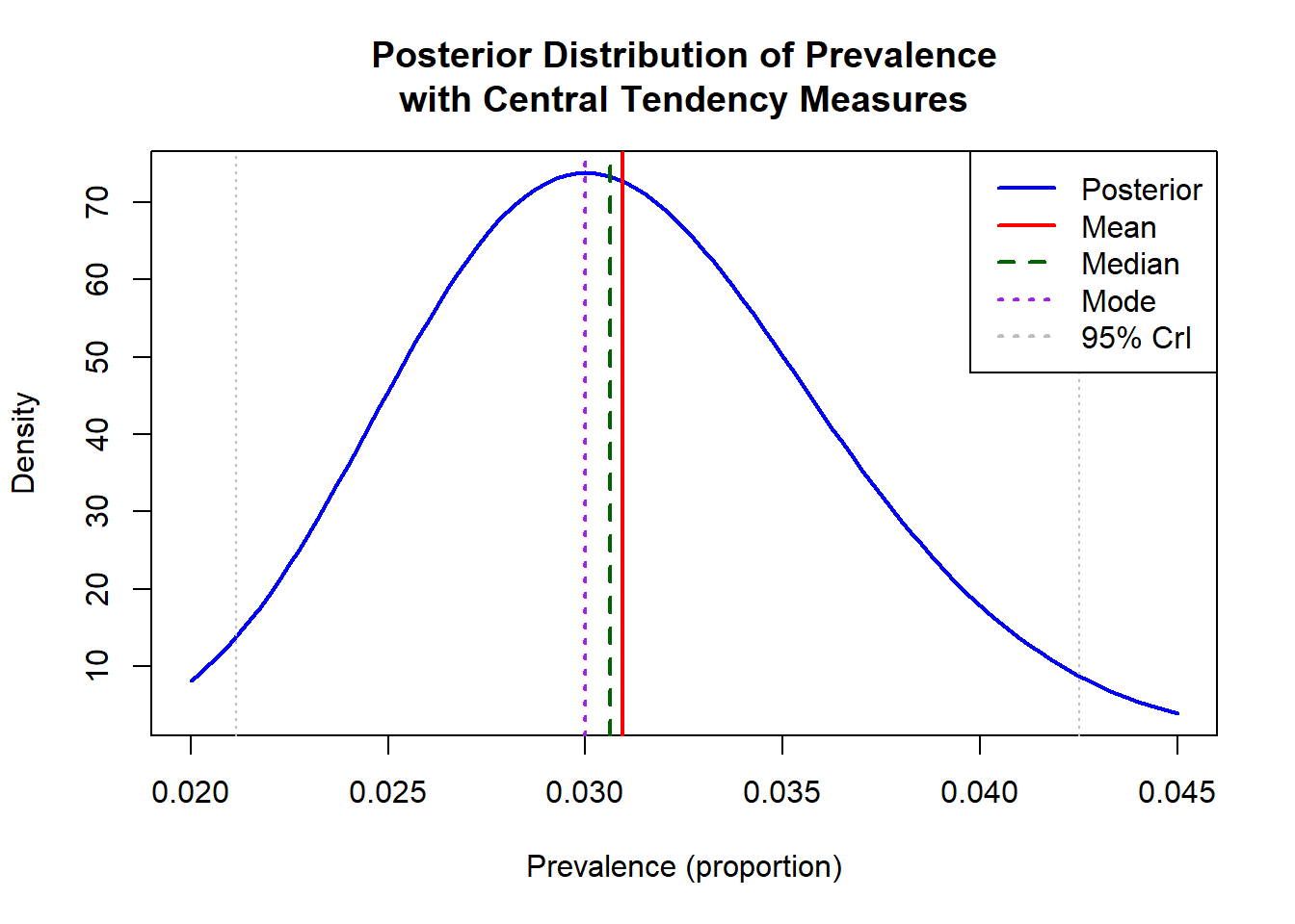
1 Mean 3.094
2 Median 3.063
3 Mode 3.000
4 95% CrI (lower) 2.114
5 95% CrI (upper) 4.251
We can plot the posterior distribution:
Code
# Use unscaled (proportion) values for plottingposterior_mean_prop <- posterior_mean /100posterior_median_prop <- posterior_median /100posterior_mode_prop <- posterior_mode /100credible_interval_prop <- credible_interval /100# Plot posterior distributioncurve(dbeta(x, alpha_posterior, beta_posterior), from =0.02, to =0.045, main ="Posterior Distribution of Prevalence\nwith Central Tendency Measures",xlab ="Prevalence (proportion)", ylab ="Density",col ="blue", lwd =2)# Add vertical linesabline(v = posterior_mean_prop, col ="red", lty =1, lwd =2)abline(v = posterior_median_prop, col ="darkgreen", lty =2, lwd =2)abline(v = posterior_mode_prop, col ="purple", lty =3, lwd =2)# Add credible intervalabline(v = credible_interval_prop, col ="gray", lty =3)# Legendlegend("topright", legend =c("Posterior", "Mean", "Median", "Mode", "95% CrI"),col =c("blue", "red", "darkgreen", "purple", "gray"),lty =c(1, 1, 2, 3, 3), lwd =2)
Now, this analysis solve our fundamental problem. We can say that
Based on the Bayesian binomial model with a uniform prior, the estimated prevalence of X disease in Montréal is 3.09% (95% CrI: 2.11%–4.25%), meaning there is a 95% probability that the true prevalence lies within this range.
However, one can now want to know that -
“What is the probability that the true prevalence of X disease is 3% or less?”
Unfortunately, we cannot get the answer of such question form our previous analyses. Fortunately, there is way to answer this question by doing Monte Carlo simulation.
        Statistic    Value
1            Mean 3.095348
2          Median 3.061198
3 95% CrI (lower) 2.097944
4 95% CrI (upper) 4.239486
Plot the results
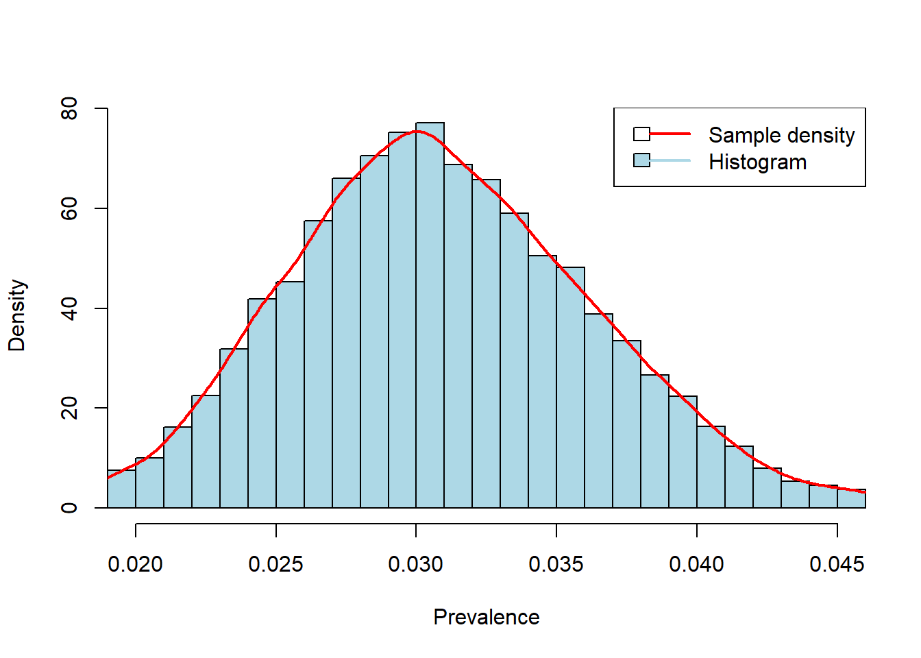
Code
# Monte Carlo histogramhist(posterior_samples, breaks =50, prob =TRUE,main =NULL,xlab ="Prevalence", ylab ="Density",xlim =c(0.02, 0.045), col ="lightblue")lines(density(posterior_samples), col ="red", lwd =2)legend("topright", legend =c("Sample density", "Histogram"), col =c("red", "lightblue"), lwd =2, fill =c(NA, "lightblue"))
Figure: Posterior distribution of prevalence.
Now, we can calculate “What is the probability that the true prevalence of X disease is 3% or less?”
Code
## Probability that prevalence <= 3%prob_leq_3 <-mean(posterior_samples <=0.03)*100prob_leq_3
[1] 45.21
We can interpret this as:
“Based on the observed data and our uniform prior, there is approximately 45% probability that the true prevalence is 3% or less.”
So far, we have learnt how Bayesian binomial model works. And we have calculated prevalence of disease X in one population. But in real world we may require to calculate the prevalence of same disease (or multiple disease) in different populations.
Let’s see, how we can do such analysis!!
For this purpose,
We will calculate prevalence of a disease, called “neurocysticercosis”, in different population using a real world data set.
We will present the results in a nice table.
Applying Bayesian binomial model with real data
Description of data set
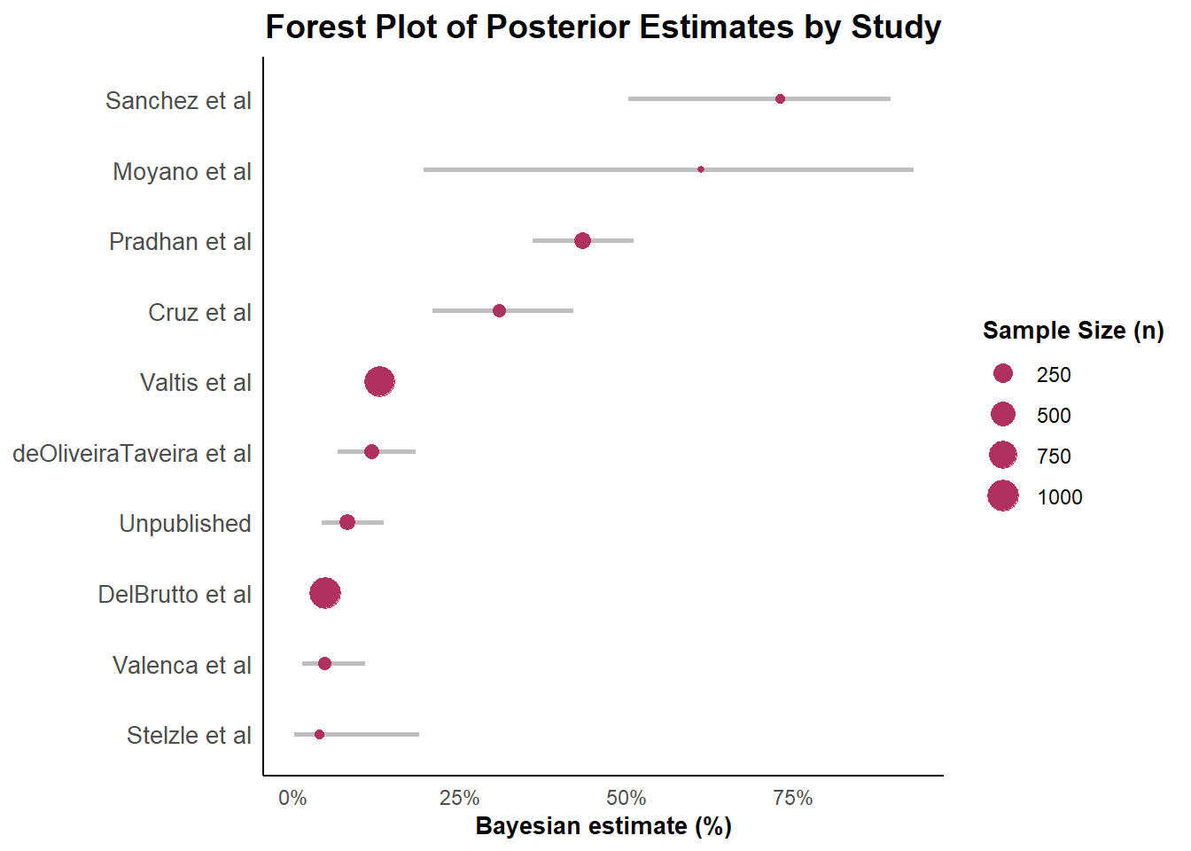
We have recently completed a brief systematic review of research articles reporting the frequency of neurocysticercosis (NCC, a parasitic disease of human central nervous system caused by the larval stage of zoonotic tapeworm, Taenia solium) among people with headache (PWH). In that review, we identified 10 studies which met the inclusion criteria (data on NCC among PWH, and NCC diagnosis was based on brain imaging). The data were organized under five variables as follows:
id: Unique ID for each study
first_author: First author
study_setting: Study setting (“Clinic_or_hospital” OR “Community”)
n: Number of people with headache manifestation who underwent brain imaging.
y: Number of NCC-cases
Code
tdat <-data.frame(id =c(500001, 500002, 500003, 500004, 500005,500006, 500007, 500008, 500009, 500010),first_author =c("Pradhan et al","Valtis et al","deOliveiraTaveira et al","DelBrutto et al","Sanchez et al","Cruz et al","Stelzle et al","Moyano et al","Valenca et al","Unpublished" ),study_setting =c("Clinic_or_hospital","Clinic_or_hospital","Clinic_or_hospital","Clinic_or_hospital","Clinic_or_hospital","Community","Clinic_or_hospital","Community","Clinic_or_hospital","Community" ),n =c(166, 924, 108, 1017, 16, 69, 17, 3, 78, 131),y =c(72, 119, 12, 48, 12, 21, 0, 2, 3, 10))tdat
       id            first_author      study_setting    n   y
1  500001           Pradhan et al Clinic_or_hospital  166  72
2  500002            Valtis et al Clinic_or_hospital  924 119
3  500003 deOliveiraTaveira et al Clinic_or_hospital  108  12
4  500004         DelBrutto et al Clinic_or_hospital 1017  48
5  500005           Sanchez et al Clinic_or_hospital   16  12
6  500006              Cruz et al          Community   69  21
7  500007           Stelzle et al Clinic_or_hospital   17   0
8  500008            Moyano et al          Community    3   2
9  500009           Valenca et al Clinic_or_hospital   78   3
10 500010             Unpublished          Community  131  10
Code
## Working data setdf <- tdat
Let’s check what are the data we have,
Code
glimpse(df)
Rows: 10
Columns: 5
$ id            <dbl> 500001, 500002, 500003, 500004, 500005, 500006, 500007, …
$ first_author  <chr> "Pradhan et al", "Valtis et al", "deOliveiraTaveira et a…
$ study_setting <chr> "Clinic_or_hospital", "Clinic_or_hospital", "Clinic_or_h…
$ n             <dbl> 166, 924, 108, 1017, 16, 69, 17, 3, 78, 131
$ y             <dbl> 72, 119, 12, 48, 12, 21, 0, 2, 3, 10
Code
head(df)
      id            first_author      study_setting    n   y
1 500001           Pradhan et al Clinic_or_hospital  166  72
2 500002            Valtis et al Clinic_or_hospital  924 119
3 500003 deOliveiraTaveira et al Clinic_or_hospital  108  12
4 500004         DelBrutto et al Clinic_or_hospital 1017  48
5 500005           Sanchez et al Clinic_or_hospital   16  12
6 500006              Cruz et al          Community   69  21
Code
summary(df)
       id        first_author       study_setting            n
 Min.   :5e+05   Length:10          Length:10          Min.   :   3.0
 1st Qu.:5e+05   Class :character   Class :character   1st Qu.:  30.0
 Median :5e+05   Mode  :character   Mode  :character   Median :  93.0
 Mean   :5e+05                                         Mean   : 252.9
 3rd Qu.:5e+05                                         3rd Qu.: 157.2
 Max.   :5e+05                                         Max.   :1017.0
       y
 Min.   :  0.00
 1st Qu.:  4.75
 Median : 12.00
 Mean   : 29.90
 3rd Qu.: 41.25
 Max.   :119.00
We see the inputs for variable “study_setting” are a bit incosistant. Let’s first check what are the inputs
Now, we want to calculate the proportion of NCC among PWH for each row of the data set and express it as a percentage along with the associated 95% credible intervals. To complete the task,
We will write a model. This is a Stan model. Then, we will compile the mode (it may take few minutes).
We will prepare our data in such way that is compatible with the model.
Then, we will apply this model to each row of our data.
We will check the convergence of the models, and results.
Model
The model assumes that the number of NCC cases \(y_i\) in study \(i\) follows a binomial distribution with study-specific sample size \(n_i\) and probability parameter \(p_i\):
A uniform \(\text{Beta}(1, 1)\) prior was specified for \(p_i\), representing an uninformative prior distribution that is equivalent to a uniform distribution over the interval \((0, 1)\).
Code
model_code <-"data{int<lower=0> N_studies;int<lower=0> n[N_studies];int<lower=0> y[N_studies];int<lower=0> alpha_prior;int<lower=0> beta_prior;}parameters {vector <lower=0, upper=1> [N_studies]p;}model{p ~ beta(alpha_prior,beta_prior);for (i in 1:N_studies){y[i] ~ binomial(n[i],p[i]);}}generated quantities{vector[N_studies] y_rep;for (i in 1:N_studies){y_rep[i] = binomial_rng (n[i],p[i]);}}"compiled_model <-stan_model(model_code = model_code)
library(here)x <-readRDS(here("Outputs","Bayesian_model_results.rds"))print(x, pars ="p", probs =c(0.025,0.50,0.975) )
Inference for Stan model: anon_model.
4 chains, each with iter=10000; warmup=5000; thin=1;
post-warmup draws per chain=5000, total post-warmup draws=20000.

      mean se_mean   sd 2.5%  50% 97.5% n_eff Rhat
p[1]  0.43       0 0.04 0.36 0.43  0.51 38436    1
p[2]  0.13       0 0.01 0.11 0.13  0.15 37357    1
p[3]  0.12       0 0.03 0.07 0.12  0.18 35724    1
p[4]  0.05       0 0.01 0.04 0.05  0.06 36390    1
p[5]  0.72       0 0.10 0.50 0.73  0.90 38862    1
p[6]  0.31       0 0.05 0.21 0.31  0.42 39721    1
p[7]  0.05       0 0.05 0.00 0.04  0.19 31598    1
p[8]  0.60       0 0.20 0.20 0.61  0.93 39946    1
p[9]  0.05       0 0.02 0.01 0.05  0.11 39272    1
p[10] 0.08       0 0.02 0.04 0.08  0.14 39839    1

Samples were drawn using NUTS(diag_e) at Thu Oct 23 00:47:51 2025.
For each parameter, n_eff is a crude measure of effective sample size,
and Rhat is the potential scale reduction factor on split chains (at
convergence, Rhat=1).
Now, check the convergence
How to check model convergence ?
In Bayesian statistics, convergence refers to two main concepts: the posterior distribution converging to the “true” distribution as data grows, and the MCMC sampling algorithm converging to its stationary distribution.
We can easily check (1) and (2) from previous chunk of code. For different plots there is an amazing function launch_shinystan() from R-package {shinystan}.
Code
launch_shinystan(x)
So far, we have calculated the prevalence proportion for multiple studies using Bayesian binomial model.
Now, we want to present the results in a nice table.